
Abstract
Belief-space planners with separately designed or off-the-shelf estimators may have access to state-relevant information the estimator does not observe. Consequently, even an estimator that minimizes mean-squared error under its own information can have a nonzero error mean when conditioned on planner information. When future corrections are intermittent and stochastic, differences between accepted and rejected error means introduce additional uncertainty terms to correction events that zero-mean assumptions ignore. In this paper, we propose a belief-space planning approach that predicts, propagates, and penalizes planner-conditioned estimator error along evaluated trajectories. A planner-conditioned estimator-error model combines affine error dynamics with a moment recursion that preserves stochastically-induced correction uncertainty. We describe a method by which to predict estimator error dynamics within specified operating regimes and incorporate predicted error moments into a task-weighted quadratic risk objective. We evaluate the approach in simulation for a tilt-rotor VTOL landing on a ship deck using receding-horizon planning. We find that conditioning on planner information reduced error-prediction loss for a command-blind EKF by 13.4% relative to a planner-ignorant model, with strongly regime and horizon-dependent forecasting abilities. In a small set of 16 paired closed-loop trials, the planner lowered the median terminal task gauge from 1.60 to 0.99, and predicted estimator error beyond 2s within a factor of 1.3, versus a 5.7-fold underprediction by covariance-only planning.
1. Introduction
Planners and estimators are often designed separately, and as such, may observe different subsets of a system’s information. In particular, planners may have limited information about the internal state representations and update procedures of “off-the-shelf" or otherwise black-box estimators, and an estimator may not receive direct information about the planner’s commands or expected future states. If the planner has relevant information the estimator lacks, an estimator with zero-mean error under its own information may have a nonzero planner-conditioned error mean. Consider the task of landing an aerial robot on a ship-deck. Deck-relative observations become intermittent over the course of the task. During these periods of intermittency, estimator error accumulates due to a lack of posterior correction availability. However, the planner may be able to partially predict this error and incorporate its predictions into trajectory design. We study the interaction between this predictable error mean and the stochastic availability of future corrections.
Conventional covariance-only belief-space planning generally assumes zero-mean estimator error. However, if nonzero-mean estimator error exists, this can have a profound impact on planner performance, as the planner will be unable to adequately predict future expected estimation error, probability of correction acceptance, or post-correction uncertainty. Additionally, when correction changes the predicted conditional error mean, stochastic correction outcomes contribute a spread-of-the-means covariance term. The resulting first two moments generally cannot be reproduced by simply inflating measurement noise to account for probabilistic observation.
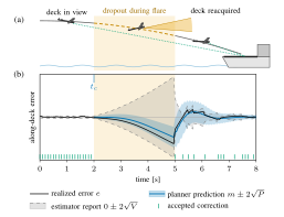
Figure 1 details and data
Predictable error through an observation dropout
Both panels share the same clock. The aircraft follows panel (a)'s authored schematic curve, with pitch interpolated between its illustrated poses; this is not measured flight motion. Panel (b) uses the paper's error samples. The aircraft holds at the drawn path's endpoint while the error plot finishes. Turn Scroll motion off to show the complete original illustration.
1.2. Contributions
We propose a belief-space planning approach which derives a model of the first and second moments of estimator error. This model is used to propagate the estimator error along candidate trajectories. The planner predicts the probability that usable corrections will be available to the estimator and moment-matches the first two error moments over both correction and no-correction outcomes at each step. This predicted error is then projected into task coordinates, from which the planner computes a task-weighted estimation risk metric. These predictions are then used by the receding-horizon planner to select trajectories.
In this work, we make the following claims:
We show that, under different information sets, even estimators that are minimum mean-squared error (MMSE)-optimal under their own information may have a nonzero planner-conditioned error mean, as established in Proposition 1 and evaluated empirically through the error prediction tests of Section 7.3;
We develop a moment-matched recursion for estimator-error propagation under intermittent corrections, capturing the additional covariance induced by separation between the accepted and rejected error means that probability-based noise inflation omits, while recovering the familiar modified-Riccati recursion in the zero-mean limit;
We formulate a task-weighted planner that penalizes predicted estimator-error moments along candidate trajectories, identify error models for three estimator architectures, and evaluate closed-loop ship-deck landing of a tilt-rotor VTOL in simulation.
We find that estimator error contains substantial planner-predictable structure when the estimator is ignorant of task-relevant information the planner holds. Prediction gains vary with forecast horizon and operating regime, though in 16 paired closed-loop trials, the proposed planner consistently improved median task performance compared to traditional covariance-only belief-space planning.
2. Information Structure and Predictable Estimator Error
At some future time , let denote the physical state and the applied command. The estimator reports an estimated state and covariance , and its estimation error is where is the difference operator on the relevant state manifold. Let denote the -algebra generated by all information available internally to the estimator at time . Each published estimator output , including , , and any other quantities published by the estimator and used by the planner-side error model, is -measurable.
The information available to the planner is (1) The planner-conditioned estimator-error moments are (2) In general, need not equal the covariance reported by the estimator.
Proposition 1 (Planner-conditioned estimator error). Let where , , and is deterministic. Then
If is -measurable, and then (3)
Proof. The MMSE property gives , and the first claim follows from the tower property. Moreover, Conditioning on under the stated assumptions then gives (3). ◻
Thus, an estimator that is MMSE-optimal given can still have nonzero error mean conditioned on when the planner has information relevant to state evolution that is not fully determined by the estimator’s information. Whether this occurs for a particular estimator and operating regime is tested from data in Section 6.
Estimates are formed using observations of the environment that arrive stochastically. In part, this stochasticity arises from sensing geometry, with the probability of successful measurement decreasing at the observer’s field of view boundaries. However, the observation of a measurement does not always lead to estimate correction. In cases where an estimator gates its accepted measurements on measurement innovation or the cadence in which measurements arrive, the probability that a measurement will be observed and that its observation will correct the estimator’s published information may partially depend on factors beyond a planner’s direct control [17]. We call the sensing and application of a measurement to a state estimate a measurement acceptance. Measurement acceptance comprises one branch of a two-branch "tree" of possible sensing outcomes that the planner must consider at each potential future correction opportunity.
3. A Planner-conditioned Model of Estimator Error
Throughout this formulation, let be the current planning time–the instant at which the planner forms a candidate control sequence and predicts forward–and denote a generic future discrete-time index along that candidate rollout. We use the subscript to denote the future time , predicted using the information available at planning time .
3.1. Planner information
The planner does not require access to the details of an estimator’s internal belief representation or propagation mechanisms in order to predict its error. However, it does require the estimator to provide a mechanism by which to initialize the error moment predictors, a model for between-correction error flow, the effect of accepted corrections on the estimator’s predictions, the probability that a correction is accepted by the estimator, and the range over which the estimator’s behavior is considered valid.
3.2. Initialization and compensation
At the beginning of planning time , the estimator-error moments are initialized using the set of all previously published estimator information using some declared initialization procedure . The planner uses this initialized error prediction to compensate the estimator’s published state, yielding a compensated planner-side state estimate , such that
(4) where is the retraction operator on the relevant manifold.
3.3. Estimator-error propagation between corrections
We model estimator-error propagation between observation-based corrections over integration interval as (5) where and characterize autonomous error evolution, collects candidate-dependent features available to the planner, and represents the retained temporally correlated residual modes. The remaining residual satisfies
Let denote correction recency, with and . Its contribution to the remaining flow uncertainty is (6) where is the baseline residual uncertainty, is the uncertainty which increases linearly with the staleness of correction channel , and is the residual uncertainty that increases quadratically with staleness. The quadratic term uses the full second-moment of stochastic recency, since
The colored residual is represented by the stable autoregressive model for with centered innovation , where is a constraint to ensure the stable decay of the latent residual state. Between corrections, recency evolves according to (7)
Define the augmented recency-error state For a fixed candidate command sequence, the between-correction estimator-error propagation model can then be written in affine form as (8) where and Its first two moments propagate as (9) and the estimator-error moments and are the -blocks of and , respectively.
3.4. Stochastic corrections
Let denote whether a usable correction occurs at rollout step . We model with (10) Here is a planner-side correction-probability model accounting for sensing cadence, trajectory-dependent sensing geometry, and conditional estimator acceptance.
Define the error of the accepted-correction branch as (11) for error-transition map and remaining correction error . For linear updates, , where is the correction gain and is the measurement Jacobian. When observations are accepted, the recency component associated with an accepted measurement type is reset to , while it continues decaying in the no-observation branch.
4. Moment Propagation Under Intermittent Corrections
Under intermittent observations of the task, future observation-based estimation corrections have state-dependent stochasticity. At each , either an observation can be accepted with probability , or the estimate can remain uncorrected and error can continue to propagate under the between-correction flow model. While branching each candidate over the possible observation outcomes would enable consideration of this stochasticity, this approach is computationally intractable for real-time control problems. We instead show that the first two moments of planner-conditioned estimator-error under stochastic observations can be matched exactly over the correction outcomes. When the prior of the predicted mean error is nonzero, this moment-matching introduces an additional covariance term, distinguishing our approach from other zero-mean treatments that rely instead on scalar noise-inflation.
4.1. Rollout assumptions
We declare the following assumptions under which we formulate our moment-matching approach.
Assumption 1 (Rollout closure). For each candidate rollout:
The local flow and correction models are evaluated only within their validated range .
Correction occurrence is conditionally independent of the realized estimator error given planner information,
Candidate command sequences are evaluated open loop between replanning updates.
4.2. Moment matching over correction outcomes
Under the stochastic-acceptance model of Section 3.4, let event denote correction acceptance at time . Likewise, denotes rejection. The first and second moments of estimator-error are defined for each branch as An exact first-two-moment closure of the branches arises from the laws of total expectation and covariance, yielding the posterior error correction model:
(12) The first two covariance terms model within-branch uncertainty, and the final term models the spread between the branch means. This final covariance term is zero precisely when the accepted and rejected branch means coincide and .
4.3. Effect of predictable estimator error
We apply this mixture to the error model established in Section 3.4. In particular, define the branch moments and . The branch is defined by (11), with resulting branch moments and .
Proposition 2 (Intermittent correction of biased error).
Let an accepted correction occur with probability under Assumption 1, and define Then the post-event estimator-error mean is (13) and its covariance is (14) where
Therefore, in general, scalar inflation alone cannot reconstruct the stochastic-acceptance uncertainty of (12).
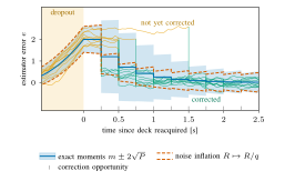
Figure 2 details and data
Possible futures after stochastic corrections
The faint sample-path markers turn from orange to green when a correction is accepted. Time advances between recorded samples without smoothing over correction jumps.
4.4. Zero-mean limit
Setting in Proposition 2 gives (15)For a linear-Gaussian correction with , , , , and (15) reduces to (16)
This is precisely a modified-Riccati update, using the familiar intermittent-measurement correction [4]. Our proposed propagation therefore contains the conventional zero-mean recursion as the special case for , with additional terms appearing only when the rejected and accepted branches have different predicted means.
4.5. Comparison with probability-based noise inflation
For the stochastic correction, define the exact expected correction map , hence . Under noise-inflated update , define . Probability-based noise inflation gives (17) For , , , and full-row-rank , (18) For (18), equality would imply , which contradicts . Its covariance update is similarly (19) which is independent of . In contrast, (20)
Therefore, since noise inflation generally mismatches the expected mean update and its covariance update is bias-independent, it cannot represent bias-dependent recursion for an arbitrary .
4.6. Recursive rollout closure
The proposed stochastic-correction recursion remains closed for the augmented error-recency state . The corresponding branch-conditioned moments are and which propagate according to (21)
5. Task-Weighted Estimation Risk and Receding-Horizon Planning
5.1. Task projection
Define the projection of estimator-error into task-relevant coordinates as (22) where is the Jacobian which maps estimator-coordinates into task-space. Let be the set of tolerances on each task axis, which defines the successful task-completion set. The task-normalized cost metric can be constructed as:
(23)
5.2. Task-weighted estimation risk
Compensation of the current physical nominal does not set , and so remains the predicted mean of the external estimator error, determining future correction outcomes and their task-space effect.
Projecting the planner-conditioned error-moments into task-space enables the computation of task-normalized estimation risk. Let the expected task-normalized estimation risk metric be defined as . Hence (24) This risk metric can be decomposed, such that for the predictable-bias risk and covariance risk . This identity is exact for the supplied moments and fixed, -measurable projection , requiring only finite second moments.
5.3. Receding-horizon planning objective
Let be the set of candidate controls from which the planner chooses. The planner evaluates candidates through open-loop recursion. Define the planner’s compensated state belief and corresponding correction-probabilities evolution as . Through bias-prediction, the first and second moments propagate according to .
Define the estimator-risk cost given the selected control as (25) Candidate controls affect through both error flow and
We define the optimal candidate selection as (26) where prices the error-compensated mean state. The first segment of the optimal policy is applied, and the replanning closes the loop at the next estimator report.
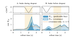
Figure 3 details and data
Compare candidate commands at a shared rollout time
Both candidates advance together. Faint markers follow the covariance-only comparison; the risk markers use the same post-correction samples as the paper.
5.4. Cross-entropy optimization
We address this planning problem using a Cross-Entropy-based receding-horizon formulation [18], [19].
When the estimator outputs information , error moments are initialized, and the planner compensates the estimates according to (4). Candidate command sequences are then sampled from a distribution. For each command tape, physical nominal dynamics and estimator-error moments are propagated, with which , , , and are evaluated. The objective of (26) is then evaluated, and the minimum-cost trajectory candidate is selected. The first command segment of this trajectory is applied, the candidate distribution is shifted for the next sampling pass, and the algorithm is repeated from the next public report.
6. Identification and Validation
A model may be constructed analytically, using known error dynamics of the system, or identified using data generated from source-trajectories. A fitted model must pass both development, selection, and closed-loop testing conditions to be considered a fully qualified error model.
6.1. Initialization and mean-error identification
At update , let be the estimator’s public innovation. Initializing from a causal affine map of the most recent innovations available at planning time , the coefficients and are fit offline on development data, to satisfy the equation: (27)
Define the between-correction rate-of-change of the estimator error
(28)
as the regression target for parameter fitting, excluding correction jumps from the fit. These correction jumps are handled separately by , , and .
The rate-model coefficients are fit to this target accordingly:
(29) which directly implies (5) under forward Euler. In particular, is the model dependence on current estimator error, is the autonomous drift coefficient, is the dependence predictable from planner-available features (e.g. command-related and recency-related features), is the temporally correlated residual structure, and is the remaining, unexplained fitting residual.
6.2. Residual covariance
After fitting the mean error dynamics model, we form the one-step residual by subtracting the model’s predicted error increment from the observed between-correction transition. The recency covariance terms are fit to the covariance of this residual, modeled by (6). The terms are fit using between-correction transitions from development data, targeting the empirical second moments and regressors , , and subject to positive-semidefiniteness constraints.
6.3. Correction and acceptance identification
For accepted-correction events, is taken directly from the estimator’s public update map when available. Otherwise, it is identified from paired pre- and post- correction errors by weighted least squares . Using the correction-noise covariance and pre-correction cross-covariance are estimated from the residual second moments. These moments are estimated within the same operating regimes used by the selected error model.
The parameters of the correction-probability mapping are fit from the binary labels using the candidate-correction samples . Known cadence or geometric components of are supplied analytically. Only unidentified components are estimated from data.
7. Shipboard landing: model identification and closed-loop evaluation
We instantiate the surrogate planning problem for landing a T1 Ranger vertical-takeoff-and-landing vehicle on a ship deck. The VTOL is represented by a 20-component state comprising position, unit quaternion, translational velocity, angular velocity, four aerodynamic-surface joint positions, and three thrust states. The seven control inputs comprise four joint-rate commands and three throttle commands. The vehicle dynamics are evaluated using an aerodynamic rigid-body model with actuator states. We then identify predictive error models for, and consider planner performance across, three independent estimators: a truth-driven estimator error-emulator, an inertial Extended Kalman Filter (EKF), and an inertial Gaussian-sum filter.
Prior work on ship-deck recovery problems assume usable state estimates and address the control and visual servoing problem presented to the planner [20], [21], [22]. We seek to investigate what happens to the estimate when the deck target leaves the sensors’ fields of regard, and how the planner should respond.
7.1. Shipboard task, dynamics, sensing, and success
Define , , and as the world, VTOL-body, and deck frames, respectively, and let map coordinates from frame into frame . The deck-relative state is defined by (30) Thus, includes the rotating-deck-frame contribution. We denote the resulting relative state by .
The aircraft state is , where contains the joint positions and the thrust states. Its dynamics are , with four commanded joint rates and three throttle inputs; the thrust states have time constant .
The planner defines the task-relative coordinates using the deck-relative coordinates above, with (31) The planner-facing estimator-error coordinates use the corresponding 12-dimensional local error where .
Simulation terminates at first physical contact between the aircraft and the ship, or planner-declared abort. Success is then evaluated using the declared acceptable landing footprint and relative landing attitude, velocities, and angular rates.
7.2. Evaluated estimators and planners
We consider three estimator architectures: E1, a truth-driven controlled-error emulator, providing a biased truth-driven estimator to the planner, for mechanism validation, E2, an IMU-driven error-state EKF with aircraft/deck navigation, gyroscope and accelerometer biases, ignorant of commands, and E3, a two-mode Gaussian sum of the inertial EKFs, for which public covariance includes between-mode spread. These estimator backends differ in how they obtain their error response coefficients, with closed-form derivation for E1 and offline fitting for the filters. Anchors are initialized using a learned affine map of the four most recent causal 12D innovations, with separately fitted residual covariance .
We additionally evaluate three planner variants: P1, our formulation, which compensates for predicted estimator error and penalizes an estimator risk metric, P2, a traditional belief-space planner for which covariance trace is the only penalized uncertainty term, and P3, a nominal-only planner. The planners are tuned identically, differing only in additional cost function terms.
7.3. Predictive error model identification and evaluation
We first evaluate whether the estimator-error model predicts error unavailable to a zero-mean model, and then whether its predicted moments are calibrated against subsequently realized estimator error.
The identified contracts exhibit strongly horizon and operating regime-dependent behavior. We therefore report prediction error by forecast horizon and trajectory regime rather than relying only on pooled loss, and discuss one of the qualified E2 error models as an illustrative case. In this model, the task-scaled mean-prediction loss was 8.16% lower than the zero-mean predictor when pooled over two experimental datasets. However, this improvement was not uniform with horizon. Over evaluation horizons of 0.25, 0.5, 1.0, and 2.0 s, the error reductions were 1.61%, 7.61%, 12.58%, and 6.39% respectively. Through the closed-loop experiments, E1 exhibited similarly horizon-dependent error dynamics to those of the identified E2 and E3 models. Along horizons of less than 0.25s, the E1 model reduced squared task-scaled prediction loss, relative to a zero-mean baseline, by 75.99%, which dropped to a 17.98% reduction between 0.25 and 0.5s, before an increase to 76.39% reduction for horizons longer than 2s.
Prediction quality also depended strongly on trajectory regime. In a separate E2 evaluation, the selected model reduced pooled prediction loss by 2.33%, but this aggregate improvement was concentrated in an operating regime with large velocities and task-relative offsets, where loss decreased by 5.52%. The same model performed worse than the zero-mean predictor during near and intermediate-range operating regimes, by 3.0% and 1.01% respectively. Hence, an error model that appears beneficial when averaged across a task distribution will not necessarily improve prediction in every portion of the maneuver. This regime dependence is particularly relevant in receding-horizon planning, because the distribution visited by the planner changes systematically as the vehicle progresses from approach to terminal alignment. These experiments show that estimator-error prediction is neither globally stationary nor characterized adequately by a single pooled accuracy or calibration metric. Predictive abilities can strengthen or reverse with horizon, transfer unevenly between regimes, and coexist with poor covariance calibration. We therefore interpret the planner-conditioned error model as a qualified local predictive model, whose claimed validity is tied to the trajectory regimes, forecast horizons, and source populations on which its mean and covariance has been evaluated.
| Estimator | Candidate | ||||
|---|---|---|---|---|---|
| E2 | Best predictive | 1.001 | 0.580 | +42.0% | +42.1% |
| E2 | Qualified | 0.739 | 0.640 | +36.0% | +13.4% |
| E2 | Zero-mean baseline | 1.000 | 1.000 | +0.0% | +0.0% |
| E3 | Best predictive | 0.846 | 0.727 | +27.3% | +14.0% |
| E3 | Qualified | 1.000 | 1.000 | +0.0% | +0.0% |
7.4. Closed-loop landing performance
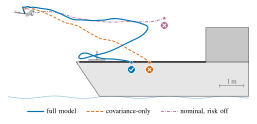
Figure 4 details and data
Replay one matched landing trial
Aircraft follow the measured simulation positions, pitch, and rotor tilt. Faint vehicles show the comparison runs; each holds its final recorded pose when its run ends.
Across 16 matched trial groups using E1, P1 achieved 8/16 physical captures, compared with 6/16 for both P2 and P3. In the paired P1-P2 comparison, P1 was uniquely successful on five trials while P2 was uniquely successful on three. Notably, P1 obtained lower component-level capture gauges than P2 in pitch and pitch rate in 11/16 trials and in longitudinal velocity in 12/16 trials. Terminal task gauge also favored planner P1, with median gauges of 0.99, 1.60, and 1.87 for P1, P2, and P3 respectively. The corresponding mean gauges were 3.69, 9.71, and 3.57, respectively, although the P2 performance mean was strongly influenced by an isolated extreme failure. Thus, the matched trials show a modest observed capture advantage and improved typical terminal task state for P1, while the available cohort remains too small to establish a difference in capture probability. Beyond 2s, P2 underpredicted realized estimator error by a factor of 5.73, whereas P1 produced an observed-to-predicted ratio of 1.31.
8. Conclusion
This work introduced a model of planner-conditioned estimator error and its evolution through intermittent observation.
Our experiments show that this error can contain substantial predictable structure, though that structure is local, with prediction accuracy and risk calibration varying strongly with forecast horizon and operating regime. While our results show modest task-success and terminal-gauge improvement over existing planning formulations, our findings indicate that predictable estimator error can be planning-relevant, but exploiting it requires modeling identification over the regimes in which the model will be used. Future work should develop adaptive or regime-conditioned models, improve calibration of long-horizon risk, and evaluate the approach over larger closed-loop cohorts and stochastic deck motion.
Acknowledgment
ChatGPT 5.6 Sol (OpenAI) was used in the preparation of this document to generate TikZ code for figures 1, 2, and 3, conduct preliminary literature reviews, format equations in LaTeX, and proofread for notational consistency and grammar. All figures, equations, citations, and text were reviewed and confirmed by the authors, and the authors claim full responsibility for the content of this work.